What Are Kirchhoff’s Laws? KCL and KVL Explained

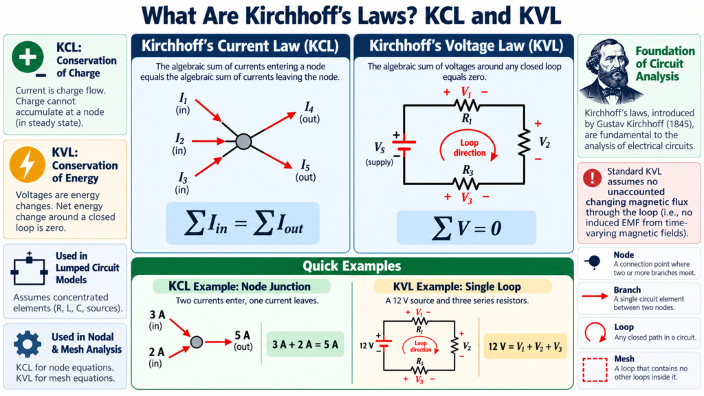
Kirchhoff’s laws are two circuit-analysis rules that express charge balance at a node and voltage balance around a loop. Kirchhoff’s current law, or KCL, relates currents entering and leaving a junction. Kirchhoff’s voltage law, or KVL, relates potential rises and drops around a closed circuit path.

These rules let you solve networks that cannot be reduced neatly to one series or parallel equivalent. They also explain why a correct answer must satisfy more than a single resistor equation. In this guide, you will learn the physical ideas, practical sign conventions, worked calculations, and assumptions behind both laws.

Kirchhoff’s laws at a glance

Law	Core equation	Where applied	Physical basis
KCL	Sum of currents entering = sum leaving	Node	Charge conservation
KVL	Algebraic sum of loop voltages = 0	Closed loop	Energy balance in the lumped circuit model

A node is a set of points joined by ideal conductors and treated as having the same potential. A branch contains a circuit element or group of elements connecting nodes. A loop is any closed path through the circuit, while a mesh is a loop containing no smaller loops in a planar drawing.

Learning these terms prevents a common confusion: a junction in a sketch is not defined merely by a dot’s appearance. Follow the wires. Points connected without intervening elements belong to the same ideal node, even when the diagram places them far apart.

Kirchhoff’s current law explained

KCL states that the total current entering a node equals the total current leaving it. An equivalent statement is that the algebraic sum of node currents is zero, provided you assign signs consistently. This is one of Kirchhoff’s laws that students use almost immediately in parallel networks.

Suppose 5 A enters a node while 2 A leaves through one branch. If only one other branch leaves, its current must be 3 A. Otherwise charge would continually accumulate at the ideal node, contradicting the ordinary steady lumped-circuit model.

KCL does not say all branch currents are equal. Their values depend on the surrounding circuit. The law specifies the balance between them. In a parallel resistor network, combine KCL with each branch’s voltage-current relationship to determine the individual currents.

What if an assumed current is negative?

Assume an unknown branch current leaves a node. If the resulting equation gives minus 1 A, the physical current is 1 A entering the node. The negative sign corrects your initial arrow; it does not make the solution unphysical.

Choosing directions before calculation is therefore safe. A consistent arbitrary choice is better than changing directions halfway through an equation. Keep the original labels and interpret negative answers at the end.

Kirchhoff’s voltage law explained

KVL states that the algebraic sum of voltage changes around a closed loop is zero in the standard lumped circuit model. Starting at a point and returning to it gives no net change in the assigned electric potential.

For a loop containing a 12 V ideal source and two series resistor drops of 4 V and 8 V, write plus 12 minus 4 minus 8 = 0. The source supplies energy per charge, and the resistors absorb the corresponding energy per charge in this ideal DC example.

Kirchhoff’s laws do not require you to travel clockwise. Either direction works. What matters is assigning a positive change when moving from lower to higher potential and a negative change when moving from higher to lower potential.

Sign conventions for resistors and sources

Across a resistor, moving in the assumed current direction produces a drop of IR. Moving against that direction produces a rise of IR. Across an ideal source, moving from its negative terminal to its positive terminal produces a positive source voltage.

A useful habit is to mark polarity on every element before writing KVL. Then your loop direction determines the sign from those markings. This is less error-prone than memorizing separate sign rules without relating them to terminal potentials.

Worked KVL example: one series loop

A 12 V ideal source feeds 2 ohm and 4 ohm resistors in series. Assume clockwise current I. Traveling from the source’s negative terminal through its positive terminal and then through both resistors gives 12 minus 2I minus 4I = 0.

Combining terms gives 6I = 12, so I = 2 A. The resistor drops are 4 V and 8 V. The sum is 12 V, as expected. The total absorbed resistor power is 2 squared times 6 = 24 W, matching source delivery of 12 times 2 = 24 W.

That power check provides an independent way to inspect the solution. It also shows that Kirchhoff’s laws work alongside Ohm’s law rather than competing with it. Each supplies a different constraint needed to describe the same circuit.

Worked nodal example using KCL

Consider a node connected to a 10 V source node through a 2 kilohm resistor and to ground through a 3 kilohm resistor. Let the unknown node potential be V. Assume currents leaving the unknown node through both resistors.

The first current is (V minus 10)/2000. The second is V/3000. KCL gives (V minus 10)/2000 plus V/3000 = 0. Multiplying by 6000 gives 3V minus 30 plus 2V = 0, so V = 6 V.

The first assumed current is minus 2 mA, meaning 2 mA actually enters the node from the 10 V source. The second is plus 2 mA, leaving toward ground. Their algebraic sum is zero, exactly as required.

Notice that a resistor current is calculated from the voltage difference between its two terminals. Using V/2000 for the first resistor would incorrectly ignore the 10 V potential at its other end. Node labels are often the simplest protection against that mistake.

A two-mesh example with a shared resistor

Imagine two clockwise mesh currents I1 and I2. Each mesh has its own 2 ohm resistor, and they share another 2 ohm resistor. The left mesh contains a 10 V source providing a rise in its clockwise direction; the right mesh has no source.

In the shared resistor, the two mesh currents oppose each other. The left-mesh equation is 2I1 plus 2(I1 minus I2) = 10. The right-mesh equation is 2I2 plus 2(I2 minus I1) = 0.

Simplifying gives 4I1 minus 2I2 = 10 and minus 2I1 plus 4I2 = 0. The second equation gives I1 = 2I2. Substitution gives I2 = 5/3 A and I1 = 10/3 A. Shared-branch current in the left mesh direction is I1 minus I2 = 5/3 A.

Mesh current is an analysis variable, not automatically the current through every component in that mesh. Shared branches carry algebraic combinations. This distinction is especially important when Kirchhoff’s laws are first used to solve simultaneous equations.

When Kirchhoff’s laws need careful interpretation

Ordinary circuit analysis assumes components can be represented as lumped elements and interconnections as ideal nodes. At high frequencies or over long conductors, propagation effects become important, and a transmission-line model may be needed.

A changing magnetic flux linked with a physical loop can induce an electromotive force. Simple electrostatic potential drops alone then do not tell the complete story. In an appropriate lumped model, induced effects are included as element voltages or sources so that circuit equations remain consistent.

KCL follows charge conservation, but a region that stores changing charge requires that storage to be accounted for. Capacitor current is included in circuit models rather than ignored. These qualifications define the model’s scope; they do not make Kirchhoff’s laws optional whenever a circuit contains AC.

A dependable circuit-analysis workflow

1. Redraw the circuit so nodes and shared branches are clear.
2. Choose a reference node and label unknown node potentials.
3. Assign current arrows and component polarities.
4. Select nodal or mesh analysis to minimize unknowns.
5. Write independent equations using Kirchhoff’s laws.
6. Solve, interpret negative values, and check power balance.

Do not count every visible loop as an independent equation. Some loop equations are combinations of others. Likewise, in a connected network with n nodes, only n minus one independent KCL equations are needed when a reference has been chosen.

Choosing between node and mesh equations

A circuit with many parallel branches often becomes simpler with nodal analysis, because each branch current can be written from node voltages. A planar circuit with relatively few meshes may be easier with mesh currents. Choose the method that produces fewer independent unknowns, then use the other balance as a check. Ideal voltage sources between unknown nodes may require a supernode; ideal current sources between meshes may require a supermesh. These are organizational techniques built from the same two laws, not additional conservation principles.

Frequently asked questions

What is the main difference between KCL and KVL?

KCL balances currents at a node; KVL balances voltage changes around a loop. Both describe the same circuit from different viewpoints. Nodal analysis emphasizes KCL, while mesh analysis emphasizes KVL.

Do Kirchhoff’s laws apply to AC circuits?

Yes, within the appropriate lumped-circuit assumptions. In sinusoidal steady state, phasor currents and voltages are used with complex impedances. In transient analysis, time-dependent element equations are used instead.

Is a negative current answer wrong?

No. It usually means the actual current flows opposite to your assumed reference arrow. Check the algebra and conventions, then report the direction clearly.

Conclusion

Kirchhoff’s laws organize circuit analysis around two balances: current at nodes and voltage around loops. With clear labels, consistent signs, and suitable component models, KCL and KVL turn complicated-looking networks into solvable equations. Practice checking the result physically as well as algebraically.